Prepping the data for mapping
In order to view the data geographically, or on a map, it needs to be matched up with geographies in the form of shapefiles. Shapefiles are the electronic files that contain not just the shape of a place, but also any data that’s associated with that place.
First we load in the libraries we need and our data.
library(readr)
library(ggplot2)
library(rgdal)
## Loading required package: sp## rgdal: version: 1.2-7, (SVN revision 660)
## Geospatial Data Abstraction Library extensions to R successfully loaded
## Loaded GDAL runtime: GDAL 2.1.2, released 2016/10/24
## Path to GDAL shared files: /Library/Frameworks/R.framework/Versions/3.3/Resources/library/rgdal/gdal
## Loaded PROJ.4 runtime: Rel. 4.9.1, 04 March 2015, [PJ_VERSION: 491]
## Path to PROJ.4 shared files: /Library/Frameworks/R.framework/Versions/3.3/Resources/library/rgdal/proj
## Linking to sp version: 1.2-4library(dplyr)##
## Attaching package: 'dplyr'## The following objects are masked from 'package:stats':
##
## filter, lag## The following objects are masked from 'package:base':
##
## intersect, setdiff, setequal, unionlibrary(ggmap)
df <- read_csv("data/all_crashData_0809.csv")## Parsed with column specification:
## cols(
## town = col_character(),
## town2 = col_character(),
## year = col_integer(),
## cycle_total = col_integer(),
## cycle_fatal = col_integer(),
## cycle_inj = col_integer(),
## ped_total = col_integer(),
## ped_fatal = col_integer(),
## ped_inj = col_integer(),
## total_crashes = col_integer(),
## total_inj = col_integer(),
## total_fatal = col_integer(),
## pop = col_number(),
## cycle_rate = col_double(),
## ped_rate = col_double(),
## total_rate = col_double()
## )Working with shapefiles
ill <- readOGR(dsn = "sixCoplaces/smaller2.shp")## OGR data source with driver: ESRI Shapefile
## Source: "sixCoplaces/smaller2.shp", layer: "smaller2"
## with 304 features
## It has 7 fieldssmaller2.shp contains places - meaning towns and other municipalities - in the six-county area. Shapefiles can be very large and detailed but the shapes in this have been simplified using a mapping program called Qgis. By simplified, we mean the shapes have been reduced in complexity - they have fewer points, which keeps the file size down.
The shapes aren’t going to be accurate to the square foot, but they’re still representative of the municipality.
Each place in the shapefile is associated with information. That information in the file can be accessed using the “@” sign instead of a “$” for dataframes. And, it’s called “data”.
head(ill@data, n = 10)## STATEFP10 PLACEFP10 PLACENS10 GEOID10 NAME10 PLACE
## 0 17 82101 02397328 1782101 Wilmington 82101
## 1 17 74275 02399944 1774275 Symerton 74275
## 2 17 69758 02399813 1769758 Shorewood 69758
## 3 17 65442 02399114 1765442 Romeoville 65442
## 4 17 64902 02399104 1764902 Rockdale 64902
## 5 17 59052 02399653 1759052 Peotone 59052
## 6 17 52584 02399470 1752584 New Lenox 52584
## 7 17 49945 02399381 1749945 Monee 49945
## 8 17 49854 02399380 1749854 Mokena 49854
## 9 17 46357 02399240 1746357 Manhattan 46357
## NAME
## 0 Wilmington city
## 1 Symerton village
## 2 Shorewood village
## 3 Romeoville village
## 4 Rockdale village
## 5 Peotone village
## 6 New Lenox village
## 7 Monee village
## 8 Mokena village
## 9 Manhattan villagesummary(ill@data)## STATEFP10 PLACEFP10 PLACENS10 GEOID10
## 17:304 00243 : 1 00428803: 1 1700243: 1
## 00685 : 1 02357470: 1 1700685: 1
## 01010 : 1 02392995: 1 1701010: 1
## 01595 : 1 02393000: 1 1701595: 1
## 02154 : 1 02393009: 1 1702154: 1
## 03012 : 1 02393010: 1 1703012: 1
## (Other):298 (Other) :298 (Other):298
## NAME10 PLACE NAME
## Addison : 1 00243 : 1 Addison village : 1
## Algonquin : 1 00685 : 1 Algonquin village : 1
## Alsip : 1 01010 : 1 Alsip village : 1
## Antioch : 1 01595 : 1 Antioch village : 1
## Arlington Heights: 1 02154 : 1 Arlington Heights village: 1
## Aurora : 1 (Other):279 (Other) :279
## (Other) :298 NA's : 20 NA's : 20We can see the shapes using the “plot” command.
plot(ill)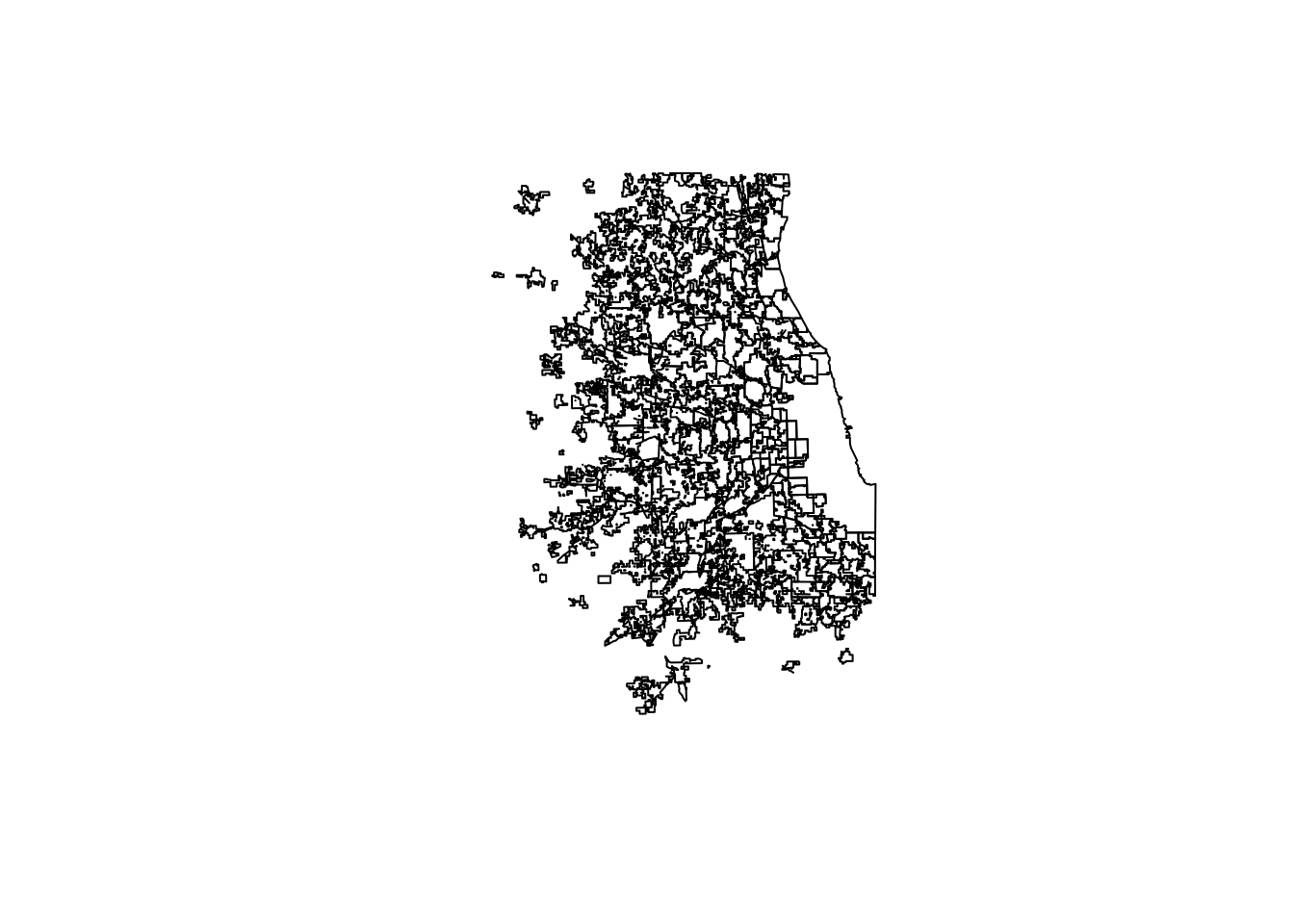
Checking the data
We can test how well our data will match up with the data in the shapefile. We’ll see if the town names in ill@data match up with the town names in our dataframe.
ill$NAME10 %in% df$town## [1] TRUE FALSE TRUE TRUE TRUE TRUE TRUE TRUE TRUE TRUE TRUE
## [12] TRUE FALSE TRUE TRUE TRUE FALSE TRUE TRUE TRUE TRUE TRUE
## [23] TRUE TRUE TRUE TRUE TRUE TRUE TRUE TRUE TRUE TRUE TRUE
## [34] TRUE TRUE TRUE TRUE TRUE TRUE TRUE TRUE TRUE TRUE TRUE
## [45] TRUE TRUE TRUE TRUE TRUE TRUE TRUE TRUE TRUE TRUE FALSE
## [56] FALSE TRUE FALSE TRUE TRUE FALSE TRUE TRUE TRUE TRUE TRUE
## [67] TRUE FALSE FALSE TRUE FALSE TRUE TRUE FALSE FALSE FALSE FALSE
## [78] FALSE FALSE FALSE FALSE FALSE TRUE TRUE TRUE TRUE TRUE TRUE
## [89] TRUE TRUE TRUE TRUE TRUE TRUE TRUE TRUE TRUE TRUE TRUE
## [100] TRUE TRUE TRUE TRUE TRUE TRUE TRUE TRUE TRUE TRUE TRUE
## [111] TRUE TRUE TRUE TRUE TRUE TRUE TRUE TRUE TRUE TRUE TRUE
## [122] TRUE TRUE TRUE TRUE TRUE TRUE TRUE TRUE TRUE TRUE TRUE
## [133] TRUE TRUE TRUE TRUE TRUE TRUE TRUE TRUE TRUE TRUE TRUE
## [144] TRUE TRUE TRUE TRUE TRUE TRUE TRUE TRUE TRUE TRUE TRUE
## [155] TRUE TRUE TRUE TRUE TRUE TRUE TRUE TRUE TRUE FALSE TRUE
## [166] TRUE TRUE TRUE TRUE TRUE TRUE TRUE TRUE TRUE TRUE TRUE
## [177] TRUE TRUE TRUE TRUE TRUE TRUE TRUE TRUE TRUE TRUE TRUE
## [188] TRUE TRUE TRUE TRUE TRUE TRUE TRUE TRUE FALSE TRUE FALSE
## [199] FALSE TRUE FALSE FALSE TRUE TRUE TRUE FALSE TRUE FALSE TRUE
## [210] TRUE TRUE TRUE TRUE TRUE FALSE TRUE TRUE TRUE TRUE TRUE
## [221] TRUE TRUE TRUE TRUE TRUE TRUE TRUE TRUE TRUE TRUE TRUE
## [232] TRUE TRUE FALSE TRUE TRUE TRUE TRUE TRUE TRUE TRUE TRUE
## [243] TRUE TRUE FALSE TRUE TRUE TRUE FALSE TRUE TRUE TRUE TRUE
## [254] TRUE TRUE TRUE FALSE TRUE TRUE TRUE TRUE TRUE TRUE TRUE
## [265] FALSE TRUE FALSE TRUE TRUE TRUE FALSE FALSE TRUE TRUE TRUE
## [276] FALSE TRUE FALSE TRUE TRUE TRUE TRUE TRUE TRUE TRUE FALSE
## [287] FALSE FALSE FALSE FALSE FALSE FALSE FALSE FALSE FALSE FALSE FALSE
## [298] FALSE FALSE FALSE FALSE FALSE FALSE FALSEThat results in a lot of “false” results, where there was no match for a place.
We ended up exporting the data and looking at it in excel. We found that all the towns in our data set match up with the towns in the shapefile. The false results were towns for which we had no data.
Reworking the data for mapping
The next problem is reworking our data so we can match it up a town.
In our dataframe, each town has up to four rows - one for each year. We need each town to have only one row to match up with the one geography.
First we grabbed the data by year
df2012 <- df[df$year == 2012,]
df2013 <- df[df$year == 2013,]
df2014 <- df[df$year == 2014,]
df2015 <- df[df$year == 2015,]
Then we renamed the columns so their names aren’t duplicated. We also deleted or nulled some unneeded columns.
df2012 <- rename(df2012,
       cycle_total_2012 = cycle_total,
       cycle_fatal_2012 = cycle_fatal,
       cycle_inj_2012 = cycle_inj,
       ped_total_2012 = ped_total,
       ped_fatal_2012 = ped_fatal,
       ped_inj_2012 = ped_inj,
       total_crashes_2012 = total_crashes,
       total_inj_2012 = total_inj,
       total_fatal_2012 = total_fatal,
       pop_2012 = pop,
       cycle_rate_2012 = cycle_rate,
       ped_rate_2012 = ped_rate,
       total_rate_2012 = total_rate
       )

df2012$town2 = NULL
df2012$year = NULL

df2013 <- rename(df2013,
                 cycle_total_2013 = cycle_total,
                 cycle_fatal_2013 = cycle_fatal,
                 cycle_inj_2013 = cycle_inj,
                 ped_total_2013 = ped_total,
                 ped_fatal_2013 = ped_fatal,
                 ped_inj_2013 = ped_inj,
                 total_crashes_2013 = total_crashes,
                 total_inj_2013 = total_inj,
                 total_fatal_2013 = total_fatal,
                 pop_2013 = pop,
                 cycle_rate_2013 = cycle_rate,
                 ped_rate_2013 = ped_rate,
                 total_rate_2013 = total_rate
)
df2013$town2 = NULL
df2013$year = NULL

df2014 <- rename(df2014,
                 cycle_total_2014 = cycle_total,
                 cycle_fatal_2014 = cycle_fatal,
                 cycle_inj_2014 = cycle_inj,
                 ped_total_2014 = ped_total,
                 ped_fatal_2014 = ped_fatal,
                 ped_inj_2014 = ped_inj,
                 total_crashes_2014 = total_crashes,
                 total_inj_2014 = total_inj,
                 total_fatal_2014 = total_fatal,
                 pop_2014 = pop,
                 cycle_rate_2014 = cycle_rate,
                 ped_rate_2014 = ped_rate,
                 total_rate_2014 = total_rate
)
df2014$town2 = NULL
df2014$year = NULL

df2015 <- rename(df2015,
                 cycle_total_2015 = cycle_total,
                 cycle_fatal_2015 = cycle_fatal,
                 cycle_inj_2015 = cycle_inj,
                 ped_total_2015 = ped_total,
                 ped_fatal_2015 = ped_fatal,
                 ped_inj_2015 = ped_inj,
                 total_crashes_2015 = total_crashes,
                 total_inj_2015 = total_inj,
                 total_fatal_2015 = total_fatal,
                 pop_2015 = pop,
                 cycle_rate_2015 = cycle_rate,
                 ped_rate_2015 = ped_rate,
                 total_rate_2015 = total_rate
)
df2015$town2 = NULL
df2015$year = NULL
With that, we joined our dated columns to the data in the shapefile. We also deleted some unneeded columns from the shapefile, saved the data and then read it back in.
ill@data <- left_join(ill@data, df2012, by = c('NAME10' = 'town'))## Warning: Column `NAME10`/`town` joining factor and character vector,
## coercing into character vectorill@data <- left_join(ill@data, df2013, by = c('NAME10' = 'town'))
ill@data <- left_join(ill@data, df2014, by = c('NAME10' = 'town'))
ill@data <- left_join(ill@data, df2015, by = c('NAME10' = 'town'))
ill@data$POPESTIMAT <- NULL
ill@data$POPESTIM_1 <- NULL
ill@data$POPESTIM_2 <- NULL
ill@data$change2010 <- NULL
ill@data$change2014 <- NULL
ill@data$change20_1 <- NULL
names(ill)## [1] "STATEFP10" "PLACEFP10" "PLACENS10"
## [4] "GEOID10" "NAME10" "PLACE"
## [7] "NAME" "cycle_total_2012" "cycle_fatal_2012"
## [10] "cycle_inj_2012" "ped_total_2012" "ped_fatal_2012"
## [13] "ped_inj_2012" "total_crashes_2012" "total_inj_2012"
## [16] "total_fatal_2012" "pop_2012" "cycle_rate_2012"
## [19] "ped_rate_2012" "total_rate_2012" "cycle_total_2013"
## [22] "cycle_fatal_2013" "cycle_inj_2013" "ped_total_2013"
## [25] "ped_fatal_2013" "ped_inj_2013" "total_crashes_2013"
## [28] "total_inj_2013" "total_fatal_2013" "pop_2013"
## [31] "cycle_rate_2013" "ped_rate_2013" "total_rate_2013"
## [34] "cycle_total_2014" "cycle_fatal_2014" "cycle_inj_2014"
## [37] "ped_total_2014" "ped_fatal_2014" "ped_inj_2014"
## [40] "total_crashes_2014" "total_inj_2014" "total_fatal_2014"
## [43] "pop_2014" "cycle_rate_2014" "ped_rate_2014"
## [46] "total_rate_2014" "cycle_total_2015" "cycle_fatal_2015"
## [49] "cycle_inj_2015" "ped_total_2015" "ped_fatal_2015"
## [52] "ped_inj_2015" "total_crashes_2015" "total_inj_2015"
## [55] "total_fatal_2015" "pop_2015" "cycle_rate_2015"
## [58] "ped_rate_2015" "total_rate_2015"write_csv(ill@data,"data/mapdata.csv")
cycped <- read.csv("data/mapdata.csv", stringsAsFactors = FALSE)
head(cycped)## STATEFP10 PLACEFP10 PLACENS10 GEOID10 NAME10 PLACE
## 1 17 82101 2397328 1782101 Wilmington 82101
## 2 17 74275 2399944 1774275 Symerton 74275
## 3 17 69758 2399813 1769758 Shorewood 69758
## 4 17 65442 2399114 1765442 Romeoville 65442
## 5 17 64902 2399104 1764902 Rockdale 64902
## 6 17 59052 2399653 1759052 Peotone 59052
## NAME cycle_total_2012 cycle_fatal_2012 cycle_inj_2012
## 1 Wilmington city 1 0 0
## 2 Symerton village NA NA NA
## 3 Shorewood village 3 0 3
## 4 Romeoville village 1 0 1
## 5 Rockdale village 1 1 0
## 6 Peotone village NA NA NA
## ped_total_2012 ped_fatal_2012 ped_inj_2012 total_crashes_2012
## 1 1 0 1 2
## 2 NA NA NA NA
## 3 1 0 1 4
## 4 9 1 7 10
## 5 NA NA NA 1
## 6 2 0 2 2
## total_inj_2012 total_fatal_2012 pop_2012 cycle_rate_2012 ped_rate_2012
## 1 1 0 5918 0.17 0.17
## 2 NA NA NA NA NA
## 3 4 0 15611 0.19 0.06
## 4 8 1 39175 0.03 0.23
## 5 0 1 1909 0.52 0.00
## 6 2 0 4703 0.00 0.43
## total_rate_2012 cycle_total_2013 cycle_fatal_2013 cycle_inj_2013
## 1 0.34 2 0 1
## 2 NA NA NA NA
## 3 0.26 1 0 1
## 4 0.26 6 0 6
## 5 0.52 NA NA NA
## 6 0.43 NA NA NA
## ped_total_2013 ped_fatal_2013 ped_inj_2013 total_crashes_2013
## 1 1 0 1 3
## 2 NA NA NA NA
## 3 1 0 1 2
## 4 3 1 2 9
## 5 NA NA NA NA
## 6 NA NA NA NA
## total_inj_2013 total_fatal_2013 pop_2013 cycle_rate_2013 ped_rate_2013
## 1 2 0 6028 0.33 0.17
## 2 NA NA NA NA NA
## 3 2 0 15906 0.06 0.06
## 4 8 1 39520 0.15 0.08
## 5 NA NA NA NA NA
## 6 NA NA NA NA NA
## total_rate_2013 cycle_total_2014 cycle_fatal_2014 cycle_inj_2014
## 1 0.50 NA NA NA
## 2 NA NA NA NA
## 3 0.13 1 0 1
## 4 0.23 5 0 5
## 5 NA 1 0 0
## 6 NA 1 0 1
## ped_total_2014 ped_fatal_2014 ped_inj_2014 total_crashes_2014
## 1 NA NA NA NA
## 2 NA NA NA NA
## 3 2 1 1 3
## 4 5 2 3 10
## 5 2 1 1 3
## 6 1 0 1 2
## total_inj_2014 total_fatal_2014 pop_2014 cycle_rate_2014 ped_rate_2014
## 1 NA NA NA NA NA
## 2 NA NA NA NA NA
## 3 2 1 16186 0.06 0.12
## 4 8 2 39675 0.13 0.13
## 5 1 1 1974 0.51 1.01
## 6 2 0 4122 0.24 0.24
## total_rate_2014 cycle_total_2015 cycle_fatal_2015 cycle_inj_2015
## 1 NA NA NA NA
## 2 NA NA NA NA
## 3 0.19 2 0 2
## 4 0.25 4 0 4
## 5 1.52 NA NA NA
## 6 0.49 NA NA NA
## ped_total_2015 ped_fatal_2015 ped_inj_2015 total_crashes_2015
## 1 NA NA NA NA
## 2 NA NA NA NA
## 3 3 0 3 5
## 4 4 0 4 8
## 5 1 0 1 1
## 6 NA NA NA NA
## total_inj_2015 total_fatal_2015 pop_2015 cycle_rate_2015 ped_rate_2015
## 1 NA NA NA NA NA
## 2 NA NA NA NA NA
## 3 5 0 16354 0.12 0.18
## 4 8 0 39774 0.10 0.10
## 5 1 0 2061 0.00 0.49
## 6 NA NA NA NA NA
## total_rate_2015
## 1 NA
## 2 NA
## 3 0.31
## 4 0.20
## 5 0.49
## 6 NACreating the dataframe for mapping
In order to use the shapefile with R’s ggplot2 graphical package, we need to process it.
ill_f <- fortify(ill, region="GEOID10")Once we do that, we need to rejoin the data we saved to the new dataframe called ill_f.
To do that, the GEOID number in the new dataframe needs to be made a number, so that we can join it with the GEOID in our data file, which is already a recognized as a number.
Then we can write the dataframe out to a csv to use for mapping.
ill_f$id <- as.numeric(as.character(ill_f$id))

ill_f <- left_join(ill_f, cycped, by = c('id' = 'GEOID10'))

write_csv(ill_f,"data/ill_f.csv")
Finally, we import and process a shapefile of the six counties. We’ll put this on top of the places layer of any map we do to make it easier to recognize where things are.
counties <- readOGR(dsn = "sixcounties/SixCounties.shp")## OGR data source with driver: ESRI Shapefile
## Source: "sixcounties/SixCounties.shp", layer: "SixCounties"
## with 7 features
## It has 5 fieldsnames(counties@data)## [1] "statefp10" "countyfp10" "countyns10" "geoid10" "namelsad10"co6 <- fortify(counties, region="geoid10")
write_csv(co6,"data/counties6.csv")